Authors: Alexander Hägele, Atli Kosson, Alejandro Hernández-Cano, Martin Jaggi

Machine Learning and Optimization Lab, EPFL.

June 15, 2026

Contact: \(\texttt{alexander.hagele@epfl.ch}\)

Figure 1: Main results of Magnitude-Direction Decoupling. Left: LR sweep. Independently of the base optimizer, fixing weights onto a sphere improves upon the optimal loss; introducing learnable magnitudes (our work, MD) gives yet another boost. Middle: Scaling laws with sparse MoEs, where improvements hold across a wide range of compute. Right: LR transfer across model width: by controlling the relative weight updates directly through the sphere, the optimal LR automatically transfers. All details are in the experimental section.

TL;DR

In this post we introduce a new optimizer tweak we call Magnitude-Direction (MD) Decoupling. We will release a more detailed pre-print about this in the coming days. This post is meant as a more approachable companion to it: it builds the intuition for the method and walks through our current experiments.

The core idea. We separate each weight matrix \(W\) into a direction \(\widehat{W}=W/\|W\|\) with fixed norm and a magnitude \(\gamma\), and learn the two separately, each updating at a well-regulated speed set by their own learning rate (LR). The magnitude need not be a single number: it can act per matrix, per row, or per row and column (which we find works best below).

The payoff. Across both Adam and Muon, decoupling magnitude and direction improves on well-tuned baselines, transfers the optimal LR across model width without retuning, and holds up as we scale to large Mixture-of-Experts models. Those results are summarized in Figure 1.

Note: Throughout, unless otherwise noted, \(\|\cdot\|\) is the Frobenius norm, and “direction” / “magnitude” may refer to the whole matrix or to its rows and columns depending on the variant.

The Problem: Magnitude-Direction Interference

We start with the following observation. A weight matrix \(W\) naturally splits into two quantities: a magnitude \(\|W\|\) and a direction \(\widehat{W}=W/\|W\|\). This is similar to specifying vectors using polar coordinates. Standard optimizers like Adam and Muon step in \(W\) as a whole, and the two quantities end up interfering with each other. Figure 2 walks through how, on a toy example.

Figure 2: Magnitude-direction interference in standard optimizers, illustrated on a toy scale-invariant loss where only the direction of the weights affects the loss. Left: the loss landscape in polar coordinates, with the same normalized optimizer step taken from a small (red) and a large (orange) starting magnitude. Middle: the identical step changes the direction — and hence the loss — far more at small magnitude than at large magnitude. Right: even though the loss has no radial gradient, the step still increases the magnitude.

The loss (left) is scale-invariant: only the direction affects the output, not the magnitude. This is a common case in deep learning, where matrices are often followed by normalization layers. Yet the magnitude still shapes what a single step does: at a small magnitude the same step changes the direction a lot, at a large magnitude barely at all (middle); and although the loss has no radial gradient, the step still grows the magnitude (right). The LR controls neither effect: directional change is governed by the current magnitude, while the magnitude drifts as a byproduct of the direction changing. This is why standard optimizers struggle to learn the magnitude of weight matrices and need weight decay to keep learning the direction in the long term. We look at both effects more closely below.

Direction change depends on magnitude. We can measure the directional change caused by an optimizer update \(\Delta W\) through the angular update \(\angle(W, W+\Delta W)\), which is closely approximated by the relative update \(\|\Delta W\|/\|W\|\). For a normalized optimizer like Adam or Muon the update size is set by the LR and is independent of the weight norm, so the directional change is roughly inversely proportional to the current magnitude \(\|W\|\) (middle panel of Figure 2). The LR therefore does not directly set the rate of directional change, and that rate can vary across layers and over time in ways that hurt learning. Our prior work on Rotational Equilibrium showed how weight decay partially fixes this by modulating the relative updates over time and balancing them across layers.

Magnitude grows despite no radial gradient. Direction changes also feed back into the magnitude. Setting aside details of momentum, updates tend to be roughly perpendicular to the current weights — from properties of scale-invariance or from noise — and a perpendicular update always increases the magnitude. This happens even when nothing pulls the weights outward: a scale-invariant function has no radial gradient, yet the norm still creeps up (Figure 2, right). For a non-scale-invariant function the (negative) radial signal has to be strong enough to counteract it. In practice the magnitudes converge toward an equilibrium set by the LR and weight decay rather than any learned optimum (see Rotat. Equilibrium), and this unnecessary growth can require tricks like Kimi’s QK-clip to tame.

Note: We describe the magnitude as a single scalar here for simplicity, but the same interference applies per row or per column: an optimizer that can’t learn the per-matrix scale well won’t do better at finer granularity.

The Solution: Magnitude-Direction Decoupling

The fix is to optimize the weight in a form that resembles polar coordinates — a direction and a magnitude — updating each separately so neither interferes with the other. Concretely, we factorize each weight into a direction \(\widehat{W}\) with a fixed norm (so it lies on a fixed hypersphere) and learnable magnitude gains:

with \(\gamma_{\text{row}}\in\mathbb{R}^{d_\text{out}}\) and \(\gamma_{\text{col}}\in\mathbb{R}^{d_\text{in}}\) learnable gains (a single scalar or a one-sided gain are special cases). The two are learned at separately controlled rates; the update rules are below.

But didn’t we just say the magnitude does not matter? Only to a point: normalization layers make the loss invariant to a single overall scalar per matrix, not to finer-grained scales. The model still needs to control the scale of its activations, amplifying some features while damping others and mixing activations that live at different scales. Per-row and per-column magnitudes change the function, and being able to learn them matters; this is exactly why the learnable gains in RMSNorm layers help. But a standard transformer has far fewer such gains than its matrices have rows and columns (and normalization layers are not everywhere), so they cannot provide the same fine-grained control. Our gains \(\gamma_{\text{row}}, \gamma_{\text{col}}\) make this control explicit and learned at a well-regulated speed, rather than through the interference-prone dynamics of the previous section.

Inside the Optimizer

Updating the direction. We keep the size of the update to \(\widehat{W}\) proportional to its magnitude, then project \(\widehat{W}\) back onto the sphere so the magnitude stays constant (relying on optimizers that produce normalized updates). The relative weight update is then determined by the LR at every step. With no equilibrium to drift toward and no dependence on the initialization norm or training length, the LR schedule directly sets the relative update.

Updating the magnitude. The magnitude of \(W\) is determined by the gains \(\gamma\), which are updated like other learnable gains typically found in normalization layers. The gains can be either a scalar, a vector acting on each row or column, or two vectors scaling both the rows and columns. We note that these magnitude gains do not provide any additional representational capacity over the original matrix; they only affect the learning dynamics.

Fused Weights. In practice, we do not want to keep \(\gamma\) and \(\widehat{W}\) separate and reconstruct the weights in the forward and backward pass. This adds unnecessary round trips through memory. Instead, the model holds the fused weight tensor \(W\) and computes the gradient \(G = \partial L/\partial W\) as usual. Then, at each step, the optimizer recovers the direction and the gain, splits the gradient between them, updates each, projects the direction back onto the sphere, and reassembles \(W\).

Let us illustrate the optimizer step in the simplest case, a single scalar \(\gamma\) with \(W=\gamma\odot \widehat{W}\):

Both gradients follow from the chain rule on \(W = \gamma \odot \widehat{W}\): the direction sees \(G\) scaled by the gain, the gain sees \(G\) projected onto the current direction. We keep the split and rescaling inside the optimizer, so the model only ever sees a “normal” weight tensor.

Reparameterized gain. Updating \(\gamma\) directly is unstable, since near zero its gradient can spike. We instead store a “raw” gain \(\widehat{\gamma}\) and pass it through a smooth map \(\gamma = \varphi(\widehat{\gamma})\), e.g. a softplus, which keeps \(\gamma > 0\) and bounds the gradient. We return to this choice in the results below; the optimal gain parametrization is still an open question.

Important Properties

• The whole idea is independent of the optimizer: the weight update can be treated as a black box, so better optimizers (AdEMAMix, Muon, Shampoo, …) should carry over.
• We no longer need weight decay, since the weights are already on the sphere. This also avoids its complicated interactions with the LR schedule, and the effective step size is now just the LR.
• We get LR transfer in width for any sufficiently long training run, because we control the relative weight update directly.
• Like Muon, we no longer need warmup, since the large early updates it exists to prevent never appear.

Decoupling Magnitude and Direction: The Details

We now present the ablations we performed along the way of finding the best recipe.

Setup. For the first part we use dense GPT-style language models from 181M to 1.29B parameters, each with head-dimension 128, GQA, QK-norm, and Sandwich Norm [1, 2]. We apply a fixed scale \(\alpha=\frac{1}{L}\) to the block-output after the RMSNorm (for proper depth scaling; more below). Matrix parameters are initialized with standard deviation \(\frac{1}{\sqrt{d}}\), and the embeddings are upscaled by \(\sqrt{d}\) to give an RMS of \(1\) going into the model. The code is a fork of Megatron-LM.

Our ablation base is the 181M model (\(d=512, L=12\)) trained on 25B tokens of a FineWeb Edu subset. This is deliberate strong overtraining (Chinchilla sense): at \(50\)k steps with a batch size of ~\(0.5\)M tokens (4096 sequence length), longer-term training dynamics become visible, closer to real pretraining runs (with millions of steps!).

We focus on AdamW and Muon as the most popular base optimizers. Across all experiments (incl. the Figure 1 sweeps), we fix the LR of every Adam-optimized parameter group at values (which we verified to be in a good range; \(10^{-3}\) for gains and output layer, \(3\cdot10^{-3}\) for embeddings) and sweep the matrix LR separately for each optimizer or setup change. This means every method is tuned with the same budget. The standard methods (AdamW and Muon) use weight decay \(0.1\); the magnitude-direction variants use none, since the weights are already on the sphere. For Muon in Figure 1 we use a scale factor of \(\sqrt{d_\text{out}/d_\text{in}}\) (which we found to be noticeably better than the RMS grafting when sweeping). Unless noted otherwise, dense models use a linear LR decay to \(10^{-8}\) for all groups. For the ablations below, we default to Muon as the matrix optimizer under MD decoupling.

Part 1: The Axes of Normalization and Magnitude

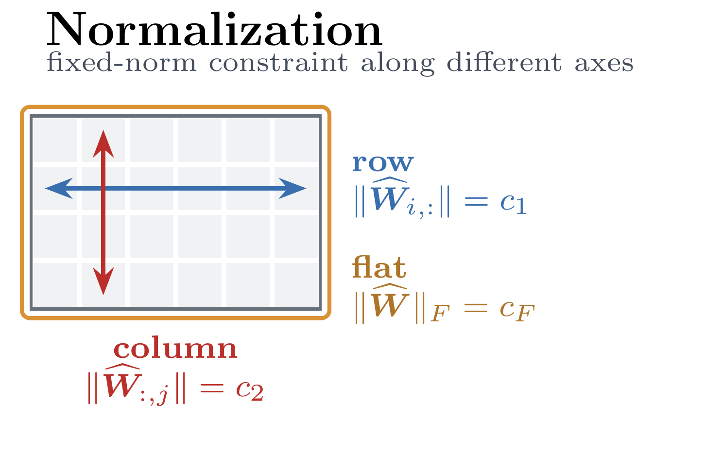
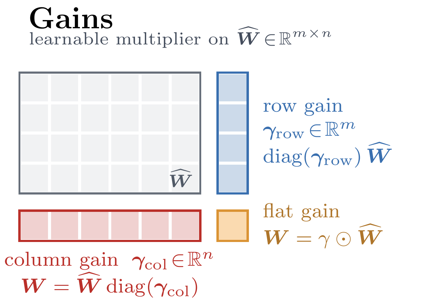
Figure 3: Illustration of the axes along which a matrix can be constrained (left), and along which gains can act (right): row, column, both, or flat / Frobenius.

There are two independent choices per matrix (Figure 3): along which axis we constrain the direction (each output row to unit norm, each input column, or the whole matrix in Frobenius norm), and along which axis the gain is free to act. We look at the normalization axis first.

Normalization axis. A priori it is unclear which constraint should work best: EDM2 keeps each row (output channel) at a fixed norm, nGPT alternates rows for QKV + up projections and columns for down projections, and AdamH/MuonH use the Frobenius norm. In each case we hold the direction at its initialization norm, so the constraint does not change the model at the start of training; with our \(\frac{1}{\sqrt{d}}\) initialization this is a Frobenius target of \(\sqrt{\max(m,n)}\) for a matrix \(\widehat{W}\in \mathbb{R}^{m\times n}\). We keep embeddings and the output (LM-head) rows at unit \(L_2\) norm throughout, independent of the sphere mode.

Note: We do not renormalize the update from the base optimizer. For Muon, we rescale its output by a fixed \(\sqrt{\max\!\big(d_\text{out}/d_\text{in},\, d_\text{in}/d_\text{out}\big)}\) so it matches the weight norm (assuming proper orthogonalization through Newton-Schulz), which we found works well. We also ablated removing the radial component of the direction’s gradient (projecting it onto the tangent space of the sphere), which made no measurable difference.

Results. Across the three constraints, the final losses turn out to be nearly identical at their optimum (Figure 4.1). Note that we do not use gains for MD in this comparison. We therefore adopt the Frobenius constraint, since it is the most flexible: it only fixes the overall scale of the matrix and leaves the relative scale of its rows and columns open.

Figure 4.1: Effect of the normalization axis: whether we constrain each output row, each input column, or the whole matrix (Frobenius) to a fixed norm. Left: LR sweep of the final loss for each normalization mode. Right: the corresponding loss curves over training.

Figure 4.2: Effect of the gain axis and its parameterization. Left: LR sweep over gain modes (scalar, per-row, per-column, or both rows and columns). Middle: LR sweep over gain parameterizations (updating the gain directly vs. through the smooth softplus map). Right: loss curves for the gain parameterizations, showing how the reparameterization avoids the loss spikes of the direct update.

Gain axis. For the gains, we compare four different settings: a single scalar, a per-row vector, a per-column vector, and a combined per-row-and-column gain (Figure 4.2, left). All of them are initialized at 1. We see a noticeable improvement of adding learned magnitudes on top of spherical training, and the combined row-and-column gain performs best. It therefore becomes our default setting. Here, all runs use the softplus parametrization described below.

Gain parameterization. Our results in Figure 4.2 (middle and right) show that the parameterization matters: updating \(\gamma\) directly produces loss spikes, because the gain’s gradient can blow up as it approaches zero. We instead pass it through the smooth softplus map \(\gamma = \varphi(\widehat{\gamma}) = \log\!\big(1 + e^{\widehat{\gamma}}\big)\) which bounds the gradient and trains stably. We are still investigating numerical strategies to understand and remove the remaining instabilities, and we have not tuned the gains’ LR, which is kept at the Adam value (here \(10^{-3}\)).

Part 2: Learning-Rate Transfer

Controlling the relative weight update directly through the spherical constraint comes with a crucial benefit: the optimal LR stays fixed as we scale the model in width, so it can be tuned once on a small model and reused on a much larger one. We are not the first to see this from a sphere / relative-update perspective: we showed the same effect with LionAR in our earlier work (Figures 19 and 20), and MuonH and HyperP report it for the Frobenius-sphere constraint with Muon. We verify that it carries over to Muon with magnitude-direction decoupling, and propose a simple recipe for depth-transfer as well.

We sweep the matrix LR while scaling the model in width, depth, and both at once, and track the relative weight update and activation statistics underlying the transfer (Figures 5.1 and 5.2).

Figure 5.1: LR transfer with Magnitude-Direction Decoupling. Left: sweep across model width. Middle: sweep across depth. Right: width and depth scaled jointly. In each panel the optimal matrix LR stays roughly fixed across model sizes.

Figure 5.2: Training dynamics underlying the LR transfer in Figure 5.1. The relative weight update is exactly controlled across width (left), which also leads to the resulting relative change in the layer's output to be stable (middle). Across depth (right) the activation RMS across the layers of a single model, showing the per-layer activation scale stays well-behaved with depth.

Results. The optimal matrix LR is essentially flat across width (Figure 5.1, left), following from the precise control of relative weight updates on the sphere (Figure 5.2, left and middle). Transfer across depth relies on the fixed block-output scale \(\alpha=\frac{1}{L}\) interplaying with the gains of the block-output RMSNorm. We have not explored better choices of \(\alpha\), but the headline is that depth scaling needs no other tricks (Figure 5.1, middle). The same transfer holds when scaling width and depth jointly (Figure 5.1, right).

Two notes. First, we transfer only the matrix LR; the embedding and output-layer LRs are held fixed across model sizes rather than scaled. Second, the transfer here is in width and depth at fixed batch size and training length. Transfer across batch size and token budget is a separate question, for which we show first experiments in the MoE section below.

For completeness, the AdamW and Muon baselines (changing only the matrix LR) are in Figure 6.

Figure 6: Baseline LR transfer for completeness, changing only the matrix LR (no magnitude-direction decoupling). Left: AdamW sweep across joint width-and-depth scaling. Middle: the same sweep with Muon.

Part 3: Learning-Rate Schedules on the Sphere

Since the relative update now follows the schedule directly (no weight decay, no equilibrium to drift toward), the shape of the decay matters more than in standard training. We compare the established recipe of a Warmup-Stable-Decay (WSD) schedule with a 20% cooldown in a negative-square-root (“1-sqrt”) shape against a simple linear decay, and look at the weight-change dynamics in Figure 7.

Figure 7: LR decay shapes on the sphere. Because the relative update follows the schedule directly, the decay shape has a clearer effect than it does under weight decay. Left: LR sweep comparing WSD and linear decay. Middle: the corresponding loss curves. Right: the relative weight update for the attention query projection follows the decay shape directly. The distortion at the very end of the right panel is an artifact of the very low LRs during the final cooldown steps.

What we see is that the established recipe no longer matches a full annealing on the sphere; in fact it is far from it. In standard, unconstrained training the weight norm grows over the stable phase, inducing an implicit LR decay even at a constant nominal LR, so a WSD schedule decays more than its nominal shape suggests. On the sphere there is no such norm growth, and the relative update tracks the schedule exactly (Figure 7, right). The optimal on-sphere schedule remains an open question, but consistent, gradual annealing appears to be the key ingredient.

Part 4: Warmup-Free and Continual Training

Decoupling removes the need for warmup: the large, destabilizing updates of the first few steps never appear, since the relative update is regulated from step one. In fact, dropping warmup even improves the loss rather than merely matching it (Figure 8, left): with warmup the early steps are wasted at a reduced LR even though training is already stable, so removing it puts them to productive use. This gain is even larger than for standard Muon.

The analogous question arises when training resumes from a checkpoint rather than from initialization (as in SFT or other post-training). To de-risk this, we run a re-warming experiment on a 150M model (Figure 8, middle and right): both the loss and the gradient norm behave well when we resume and re-warm, even when we reuse the optimizer state and use no warmup. Staged and continual training therefore do not seem to be a problem. The impact of decoupling on properties such as sharpness is an interesting question for further study.

Figure 8: Warmup-free and continual training. Left: LR sweep with and without warmup, showing dropping warmup improves the loss. Middle: loss curves for re-warming runs on a 150M model. Right: the gradient norm over the same re-warming runs, confirming training stays stable.

Part 5: Scaling Up to Large MoEs

Setup. We now turn to Mixture-of-Experts (MoE) transformers in Megatron to check that our improvements persist at scale. Sizes range from 1.2B-6.7B total and 270M-810M active parameters, at a fixed 6% non-embedding sparsity with 64 experts (1 shared) and top-2 routing. Unlike the dense models above, these do not use RMSNorms after the attention and MLP blocks (simply because this experiment started in a different codebase of Megatron). We train on the Apertus 1.0 phase-5 data mixture (DCLM-edu, FineWeb-2 HQ), a good mixture for verifying routing in multilingual settings.

The recipe has three steps: find the optimal LR on a small base model, transfer it to larger models with a scaling rule, and then scale up and compare.

Step 1 — find the optimal LR. We fix a base model at 270M-active / 1.2B-total and train for ~15B tokens (28k steps), sweeping the matrix LR for each optimizer individually (Figure 9, left). As before, the remaining LRs (embeddings, LM head, gains) are held fixed at \(10^{-3}\) with Adam, and the standard methods use a weight decay of \(0.1\), so each optimizer is tuned with the same budget on a shared base. For Muon we use a shape-scaling factor of \(\max\!\big(1,\ \sqrt{d_\text{out}/d_\text{in}}\big)\); the lower bound of 1 matters so the router is not given a much downscaled LR. For MuonMD we additionally normalize the routers along the expert axis (rows), otherwise following the earlier recipe.

Step 2 — transfer it to larger models. With the optimal matrix LR fixed from the base sweep, we scale up without re-tuning. For the AdamW and Muon baselines we follow the Complete(d)P parametrization to set the LR and weight decay for all parameter groups across model width and training length. For MuonMD the recipe is simpler: because the sphere constraint already gives LR transfer across width (Part 2), we need no width multiplier at all and only have to account for the training length. There we scale LRs by \(1/T^{0.25}\) (\(T\) the token-count scaling factor), gentler than Complete(d)P’s \(1/T^{0.5}\) on the nominal LR, motivated by our intuitions from rotational equilibrium, where the effective LR \(\sqrt{\eta\lambda}\) governs the dynamics.

Note: The right exponent for scaling the LR with training length is still unsettled; other works report values around \(0.3\) (e.g. HyperP). A principled choice for the sphere setting, where the LR directly sets the relative update, remains open. We briefly verified that \(0.25\) works better than \(0.5\) for MD training, but have not studied it exhaustively yet.

Step 3 — scale up and compare. Putting it together, we scale to the large MoEs and compare against the baselines transferred from the tuned base (Figure 9), varying dataset size \(D\) from 7.5B-44B tokens. For the scaling law we plot loss against compute measured as non-embedding active-parameter FLOPs, i.e. \(6\,N_\text{act}\,D\) with \(N_\text{act}\) the number of active non-embedding parameters. For the third experiment we reuse the 270M-active / 1.2B-total base config and increase the batch size by \(k\) while scaling the LR by \(\sqrt{k}\).

Figure 9: Putting it together in large MoEs. Left: LR sweep of different base optimizers. Middle: scaling law of loss vs. compute (FLOPs), where the improvement holds across a wide range of compute. Right: batch-size scaling as a function of the global batch size.

Results. The gains from decoupling persist at scale and in the MoE setting, where MuonMD improves on tuned Muon and AdamW (Figure 9, left). When scaling models and training lengths, MuonMD stays ahead across the full range of compute we tested, reaching AdamW’s loss with roughly \(2\times\) less compute (Figure 9, middle). This advantage holds across global batch sizes (Figure 9, right).

A few caveats. Our protocol is principled, but certainly imperfect.

• The Adam-group LRs were not separately tuned, and the initial values might be suboptimal (which would spill into other configurations).
• We did not verify that Complete(d)P holds exactly in our setting or how it changes with Muon, and we did not apply the depth scaling rules. Still, it represented the most rigorous approach accounting for the different axes of scaling without spending large compute on tuning.
• We initially kept a short warmup for Muon, assuming it helps the Adam-optimized parameters not held on a sphere, but this no longer seems to be the case (see above).
• When varying the training tokens across models, we did not change the batch size or iteration count, which might change the compute-optimal scaling.

Our WandB is publicly accessible for both dense and MoE runs.

Related Work

This work is a follow-up to Atli Kosson’s thesis, On Balanced Representation Learning in Neural Networks (2026), which contains broader discussions and references. There is a rich and fast-growing body of related work; we have tried to be exhaustive below, so if we missed something, please reach out.

Most recent and directly related. A handful of very recent works share our core motivation of decoupling, learning, or constraining the magnitude of weight matrices when training with Adam or Muon:

• AdamH / MuonH (2026) constrain the weights to a fixed Frobenius sphere and drop weight decay, like our direction update. HyperP (2026) builds on top of this and investigates how to achieve LR transfer across width, depth, training tokens, and MoE granularity. However, both keep the norms fixed, but add no learnable magnitude gains. While RMSNorm gains keep a certain expressivity, we find that adding explicit per-row/per-column gains on top helps more.
• Muown (2026) reparameterizes each weight into a per-row magnitude and a directional factor (a similar separation as ours, limited to rows), updating the magnitude with Adam and the direction with Muon, motivated by Muon’s tendency to let the spectral norm drift upward. Unlike ours, it does not keep the direction on a fixed norm, but lets them grow at each step. This leads to an implicit LR decay for growing weights.
• Learnable Multipliers (2026) and Scale Vectors (2026) both learn explicit scales, similar to us; the former adding scalar/per-row/per-column multipliers to each matrix, the latter studying the scale vectors in normalization layers and proposing a magnitude–direction reparameterization. Neither holds the weights at a fixed sphere norm.

Sphere and manifold constraints for LLM training. A connected line of work constrains the weights (and sometimes updates) to a sphere or matrix manifold during pretraining, differing mainly in which norm is fixed and whether magnitude is added back. On a per-vector or Frobenius sphere: nGPT (2024) normalizes every weight’s rows/columns (depending on up/down projection) as well as activations to a fixed L2 norm of 1 (different to RMSNorms); anGPT (2025) relaxes this to an approximate norm constraint; Nemotron-Flash (2025) keeps the nGPT unit-norm projections without the other architectural changes; and Mano (2026) projects the momentum onto the tangent space of a rotational oblique manifold (alternating unit-norm columns and rows). On the spectral norm instead: SSO (2026) constrains both weights and updates, Modular Manifolds (2025) co-designs the optimizer with a Stiefel constraint, and Enforced Lipschitz Constants (2025) bounds the operator norm throughout training. We instead fix the softer Frobenius norm and add learnable magnitudes inside the optimizer, independent of how the update step is obtained. Relatedly, width scaling under operator norms (2026) obtains the same LR transfer from an operator-norm view, while Target Variance Rescaling (2025) periodically rescales to a target variance rather than a norm.

Controlling the relative update. Previous work aims to control the update size relative to the weight, without an explicit magnitude/direction split. We previously argued that controlling the relative weight update is the main effect of weight decay, creating Rotational Optimizer Variants (RVs, 2023) and LionAR that achieve the same effect by fixing the weight norm and scaling the update norm to be proportional on average. Nero (Liu et al., 2021) was an earlier optimizer that used a similar mechanism of constraining the norms and controlling the update norm of each neuron without specifically relating it to weight decay. LARS (2017) and LAMB (2019), and variants of AdaFactor (2021) scale the update of each layer to be proportional to the weight norm without explicitly constraining it. In RL, Normalize-and-Project (2024) periodically projects weights back to their initial per-layer norm to keep the effective LR constant — our sphere constraint, motivated by plasticity rather than transfer. For diffusion models, EDM2 (Karras et al., 2023) combines weight projections and normalization layers to keep relative updates from decaying over time and balance their size between layers. AdamP / SGDP (2021) removed the radial component of the update stemming from momentum to slow down the magntiude growth without explicitly constraining the norm.

Classic reparameterization and normalization. The idea of separating a weight’s magnitude from its direction goes back to before LLMs:

• Weight Normalization (Salimans & Kingma, 2016) reparameterizes each weight as \(w = (g/\|v\|)\,v\) — a learnable scalar magnitude \(g\) times a direction. This is the most direct classic ancestor of our gains, though without a fixed-norm constraint or a separate LR for the direction.
• Decoupled Networks (2018) factor the neuron’s inner product into a magnitude function times an angular function of the angle between weight and input.
• Weight Standardization (2019) and its use in BiT (2020) standardize the weights feeding each output channel to zero mean and unit variance to smooth the loss landscape, and Spectral Normalization (Miyato et al., 2018) divides each matrix by its top singular value to bound the Lipschitz constant in GANs. Hyperspherical units, e.g. AKOrN (2025), keep their state vectors on a sphere by construction.

These methods normalize or reparameterize weights for conditioning, stability, or robustness. Our contribution is to put the direction on a fixed sphere with a normalized update and learn per-row/per-column magnitudes at their own rate, specifically to remove the magnitude–direction interference and improve training performance.

Discussion

Magnitude-direction decoupling is a simple change that pays off across optimizers and scales. We leave a careful accounting of the per-step overhead for the pre-print: in our experiments it is minimal, and we are currently building a distributed implementation that overlaps the projection and reparameterization with existing computation and communication, which should eliminate it entirely.

The best way to parametrize the magnitude and direction is still open, as is the parametrization of the gains. MD training also opens interesting questions about the sharpness of the loss landscape and about downstream behaviour, in particular RL.

Acknowledgements

This work used compute from the Swiss AI Initiative on the Alps cluster under the Apertus initiative. We thank Fabian Schaipp, Mikhail Gorbunov, and Skander Moalla for helpful discussions.

Citation

@misc{hagele2026improving,
  title={Improving Neural Network Training by Decoupling the Magnitude and Direction of Weight Vectors},
  author={H\"agele, Alexander and Kosson, Atli and Hern{\'a}ndez-Cano, Alejandro and Jaggi, Martin},
  year={2026},
  url={https://haeggee.github.io/posts/magnitude-direction-decoupling}
}